I was recently asked by my good friend John Marshall, the longest serving Visio MVP (see http://visio.mvps.org/ ), if I had any examples of using arrays in shapes, rather than having scores of Shape Data rows. Indeed, I have used arrays in many shapes, and used the LOOKUP() and INDEX() ShapeSheet functions to extract discreet values, but I thought I would enhance an existing shape, the Pie chart master on the Charting shapes stencil to demonstrate a technique.
In this post, the screenshots are from Visio 2010, and I have used the Link Data to Shapes feature that was introduced in Visio 2007, but a similar effect can be done using the Database Wizard which has been part of Visio since version 4.1 back in 1997.
I started a new Business Charts and Graphs diagram, and dragged a dropped a Pie chart master on to the page. This shape allows for the user to enter values for 1 to 10 pie slices by use of the right mouse menu.
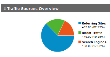
Next, I need some data, so I decided to use the website traffic from Google Analytics for three different websites.
I entered the values into an Excel table, and created a formula in column H (Slice) that concatenates the values from columns D to G together with a “@” character as a separator.
I then created another table that referenced values in the first table. This time I concatenated the values in the relevant rows of the first table with the “|” character.
 So, now I effectively have an array for each slice inside an array for the each of the three pies.
I saved the Excel workbook as PropertyArray.xlsx
The next task is to Link Data to Shapes in Visio to get the, and use the PieTitle, PieSubject and PieDescription columns as the unique identifiers. I also defined the PieSubject column as hyperlink text.
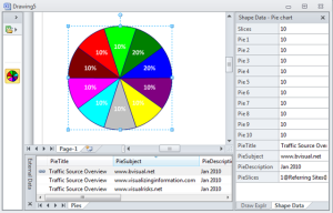
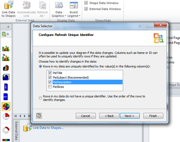 So now I have three rows in my External Data window, and the PieSlices column contains my array of arrays.
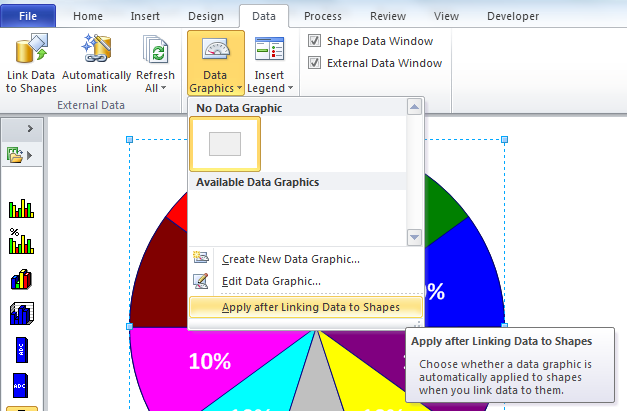
 Next, I checked that the automatic Data Graphics / Apply after Linking Data to Shapes option is un-ticked … I don’t want any Data Graphics.
 So now we have a pie shape which has all of the data, but it does not behave correctly
If we now turn our attention to the ShapeSheet of this shape, we can see that four new Shape Data rows have been added, along with an Hyperlink. Our array has gone into the Prop._VisDM_PieSlices.Value cell.
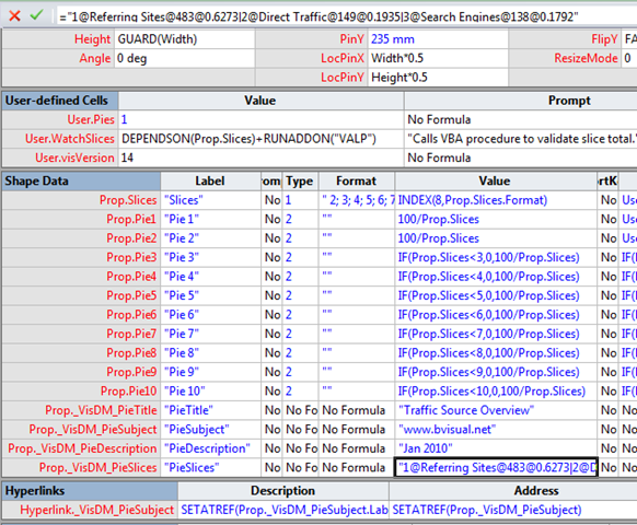 So, now we just need to modify some of the other cells to refer parts of this array.
The Prop.Slices.Value cell determines how many slices there are, so wouldn’t it be neat if we could count the number of slices from our array? Well, we can!
The text uses the “|” character to split the pie into slices. Therefore, the formula LEN(INDEX(n,Prop._VisDM_PieSlices,"|")) will find the nth slice. Note INDEX is zero-based therefore the first slice is INDEX(0,….). Now, if there isn’t a slice present, then this formula will return an empty string, thus LEN(..) will return 0, otherwise it will return the number of characters found. So, if you then enclose the formula with ABS(…) you will get 1 or 0. Therefore, the following formula in Prop.Slices.Value cell will simply add 1 or 0 for each pie slice, ending up with the total number of slices, in this case 3:
=ABS(LEN(INDEX(0,Prop._VisDM_PieSlices,"|"))>0)+ABS(LEN(INDEX(1,Prop._VisDM_PieSlices,"|"))>0)+ABS(LEN(INDEX(2,Prop._VisDM_PieSlices,"|"))>0)+ABS(LEN(INDEX(3,Prop._VisDM_PieSlices,"|"))>0)+ABS(LEN(INDEX(4,Prop._VisDM_PieSlices,"|"))>0)+ABS(LEN(INDEX(5,Prop._VisDM_PieSlices,"|"))>0)+ABS(LEN(INDEX(6,Prop._VisDM_PieSlices,"|"))>0)+ABS(LEN(INDEX(7,Prop._VisDM_PieSlices,"|"))>0)+ABS(LEN(INDEX(8,Prop._VisDM_PieSlices,"|"))>0)+ABS(LEN(INDEX(9,Prop._VisDM_PieSlices,"|"))>0)
Next, we want to have the percentage value of each slice in the relevant Prop.Pien.Value cell. We know that INDEX(n,Prop._VisDM_PieSlices,"|")) will get the array of values in each slice, so INDEX(3,INDEX(n,Prop._VisDM_PieSlices,"|"),"@") will return us the fourth part of the array, split with the “@” character, in the nth pie slice. We know from our spreadsheet that this is the percentage value, so we just need to multiply by 100 for this shape to automatically size. Thus the formula for Prop.Pie1.Value is:
=IF(LEN(INDEX(0,Prop._VisDM_PieSlices,"|"))=0,0,INDEX(3,INDEX(0,Prop._VisDM_PieSlices,"|"),"@")*100)
Similarly, the Label and Prompt formula can be set to display the SliceName and SliceValue values.
Prop.Pie1.Label=INDEX(1,INDEX(0,Prop._VisDM_PieSlices,"|"),"@")
Prop.Pie1.Prompt=INDEX(2,INDEX(0,Prop._VisDM_PieSlices,"|"),"@")
You can simply copy and paste these formulae into the other Shape Data rows, and amend the second INDEX position in each row to suit:

In fact, you can also amend the ScreenTip of each pie slice shape by opening up each of their ShapeSheets to enter a formula in the Miscellaneous Comment cell. Notice that this formula must include the Sheet.n! of the parent Pie chart shape. (It will be Sheet.1 if you only have one shape on your page … it is usually Sheet.5 if you are editing a master shape).
 Well, now we are getting close to our desired result:
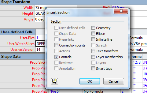
 The Pie chart shape has a text block below it, but I was rather that its position can be changed by moving a Control handle. So, open up the ShapeSheet (if it isn’t still open), and Insert the Controls section:
So, edit the RowName, X and Y values to Label, =Width*1.5 and =Height*1 respectively:
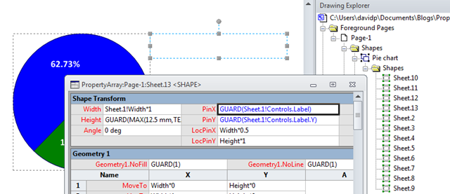
 Next, use the Drawing Explorer window to locate the text block sub-shape in the Pie chart shape. Open up its ShapeSheet and amend the PinX and PinY formulae to reference the X and Y position of the control handle that we have just created.
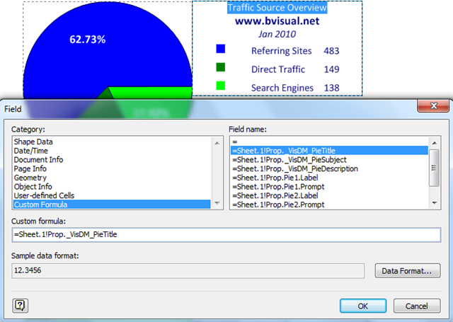
All that remains is to edit the text block to contain the legend of the pie chart. We can use Insert Field to add custom formula, but note that we must type in the values with the parent shape NameID again, in this case Sheet.1!.
For the slice rows, you can insert a symbol (I chose a Wingdings one); tab; =Sheet.1!Prop.Pie1.Label; tab and =Sheet.1!Prop.Pie1.Prompt per row.
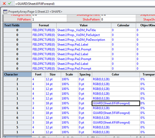
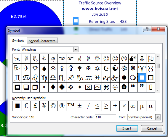 Obviously, this does not set the color of the symbol, but Visio is really cool because we can just open up the ShapeSheet of the text block, locate the relevant row in the Character section., and enter a reference to the FillForeground cell of relevant pie slice shape:
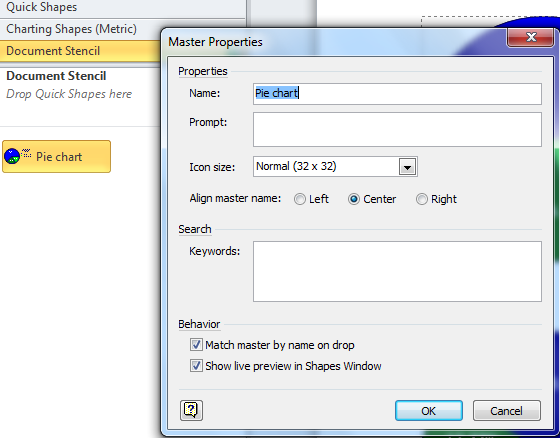
Finally, we can delete the original Pie chart master on our Document stencil; drag our Pie chart shape onto the Document stencil; re-name as Pie chart and ensure that Match master by name on drop is ticked.
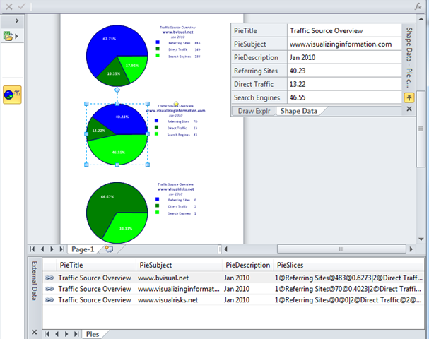
 Well, we eventually have it … a smart Pie chart shape that can be linked to to a data source, and refreshed.
 John .. I hope that answers your question about how to use an array in Visio shapes?
Download the Visio and Excel documents here : PropertyArray.zip



I would like to create a 3D Histogram with two 3D circles… I think given the capabilities of Visio… it should be able to do so easily… can you help please? This is what I mean -> http://www.youtube.com/watch?v=P2PtA7cFDt0&feature=results_main&playnext=1&list=PLDF6950F0D5795590
Have you looked at the General / Block Diagram with Perspective template?
You could probably adapt them to do something similar
Yep looked at it. But it really means having to manually calculate all the pie ratios and make a chart out of it… Whereas if there were a 3D pie chart that would simply make the chart based on an Excel range and save like *days* of time 🙁
Thank you for the plug. I am currently looking at another application where this may apply.
I come up with some strange Visio ideas and you or one of the other Visio MVPs have a solution.